“When captured electronically, customer sentiment — expressions beyond facts, that convey mood, opinion, and emotion — carries immense business value. We’re talking the voice of the customer, and of the prospect, patient, voter, and opinion leader.” – Seth Grimes

Sentiment analysis is the computational study of opinions, attitudes, and emotions expressed in (written) language, and is commonly used in natural language processing to determine the polarity of a text as expressing positive or negative sentiment. This project follows as: four NLP models — CNN, RNN, RCNN, LSTM — were trained and tested on the Large Movie Review Dataset v1.0 and compared for their metric scores — loss, accuracy, F1 macro and micro, missclassification rate, training time — across ten epochs controlled for validation loss. Each epoch’s performance is tracked and averaged.

Model		Loss		Accuracy		F1macro		F1micro		Mis. rate		Training time (s)
CNN		0.50		0.83		0.83		0.83		0.17		14.56
RNN		0.48		0.83		0.83		0.83		0.17		36.29
RCNN		0.50		0.83		0.83		0.83		0.17		87.49
LSTM		0.38		0.84		0.84		0.84		0.16		114.31

An ideal model will minimize validation loss, misclassification rate, and training time while maximizing accuracy and F1 scores. Following from average scores, we see that a minimized loss and misclassification rate with best performing accuracy and F1 scores follow for the LSTM model, though optimized for time follows for the CNN model.

The visualization and neural network models used in this project are available here.

Introduction

One task in natural language processing is so-called opinion mining, or sentiment analysis. One task in particular in sentiment analysis is polarity, in which we analyze a text and process whether the information it entails has positive or negative sentiment (Bodapati et al., 2019).

Traditional text classification methods were exhasutively dictionary-based and required much computing power or employed basic machine learning methods; recently, more efficient and accurate deep learning methods such as LSTM (Long Short-Term Memory) models have superseded them (Jang et al., 2020), and likewise for any of the species of BERT (Bidirectional Encoder Representations from Transformers) models (Hoang et al., 2019). This project aims to explore and compare various models for polarity sentiment analysis for the following reasons: learn machine learning methods for text classification; learn about optimization methods for machine learning; learn to apply text analyses for further research.

The problem posed in this project is that of binary classification of polarity: determination of whether a review is positive or negative. The Stanford IMDB dataset is used for the experiment, which consists of movie reviews classified as positive or negative. Four kinds of ML models are compared for their performance in predicting polarity. The question remains: what models yield best metric scores for polarity sentiment prediction?

Methods

The Stanford IMDB review dataset (Maas et al., 2011) is a repository of training and testing data consisting of 50000 reviews. Out of the total records, 25000 are of positive polarity while the other 25000 are of negative polarity. 12500 positive reviews and 12500 negative reviews are in each of the training and test data.

The review dataset is cleaned for stopwords, punctuation, and contractions, and is otherwise normalized to facilitate meaningful comparisons. Each model follows the same general schematic template with some variation (descriptions here follow exactly from the Keras documentation): sequential model is appropriate for a plain stack of layers where each layer has exactly one input tensor and one output tensor; embedding layer turns positive integers (indexes) into dense vectors of fixed size; dropout layer randomly sets input units to 0 with a frequency of rate at each step during training time, which helps prevent overfitting; 1D convolution layer creates a convolution kernel that is convolved with the layer input over a single spatial (or temporal) dimension to produce a tensor of outputs; dense layer is a layer that is deeply connected with its preceding layer which means the neurons of the layer are connected to every neuron of its preceding layer; LSTM layer includes many LSTM units to recall past information; output does just that; compile gives specifications about the model such as optimization, minimization of error, and which metrics to evaluate and report.

Architecture		CNN		RNN		RCNN		LSTM
sequential		✓		✓		✓		✓
embedding		✓		✓		✓		✓
dropout		x		✓		✓		✓
convolutional		✓		x		✓		x
dense		✓		x		x		x
LSTM		x		✓		✓		✓ (multiple)
Output		✓		✓		✓		✓
Compile		✓		✓		✓		✓

Each model is constructed with training epochs monitored for validation loss as the criteria for early stopping. Because too many epochs can result in an overfitted model that fits exactly against training data, which results in the model inaccurately performing against novel data, thus defeating its purpose. Loss quantifies how certain the model is about a prediction, whereas accuracy checks for the number of correct predictions (Kelleher et al., 2015). It follows, then, that stopping for loss on the validation set will best prevent overfitting.

To optimize completion time, each model was forced to perform on the GPU via the CUDA Toolkit. The GPU used is NVIDIA GeFORCE RTX 3070. Preliminary tests were done on the CPU: AMD Ryzen 7 3700X 8-Core Processor 3.59 GHz. Final results reported in this paper are those run on the GPU. To force the LSTM model to run on the GPU via CUDA, we do so via cuDNN.

Results

n-gram analyses for n={1, 2, 3} is visualized below. n-grams track the frquency in which (word) tokens appear. 1-grams (monograms) refer to the frequency in which single word tokens appear; 2-grams (bigrams) refer to the frequency in which two word tokens appear together; 3-grams (trigrams) refer to the frequency in which three word tokens appear together. Roughly, such frequencies will follow a Zipf-like distribution. n-grams are useful in that they tell us exactly word distributions (once appropriately filtered). Word pairings are exceptionally useful in many contexts, not limited to sentiment. Reconstruction of broken or incomplete texts, for example, and auto-correct are applications of n-grams. The n-gram distributions are plotted accordingly.

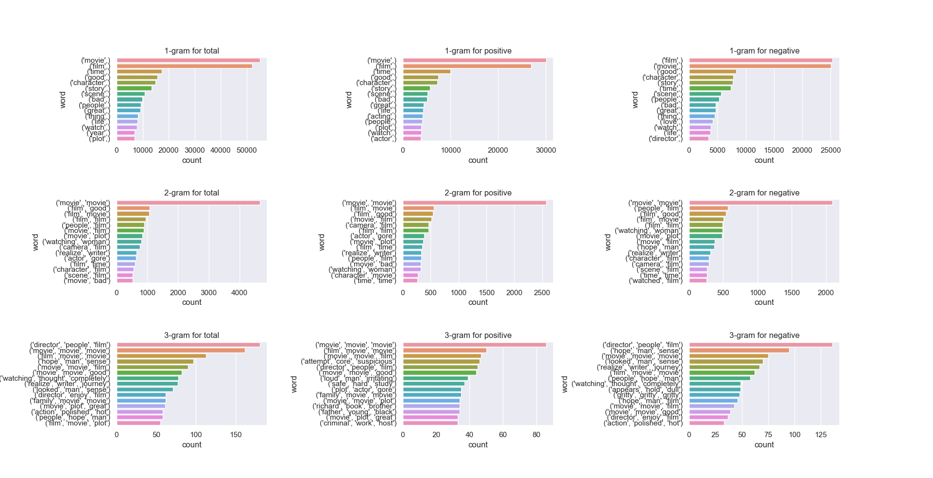
Other visualizations such as wordclouds, number of characters in cleaned texts, number of words in cleaned texts, and average word length in cleaned texts are provided in the appendices.

An ideal model will minimize validation loss, misclassification rate, and training time while maximizing accuracy and F1 scores. The following graph shows such measurements for the CNN model as an example, while the remaining models are given in the appendices.

Interestingly, even when forcing the model onto the GPU, the LSTM is markedly temporially expensive. This expense follows from the sequential computation of the LSTM layers. We can compare the training times of each model graphically via a quick script display.py that is hardcoded for comparing training times.

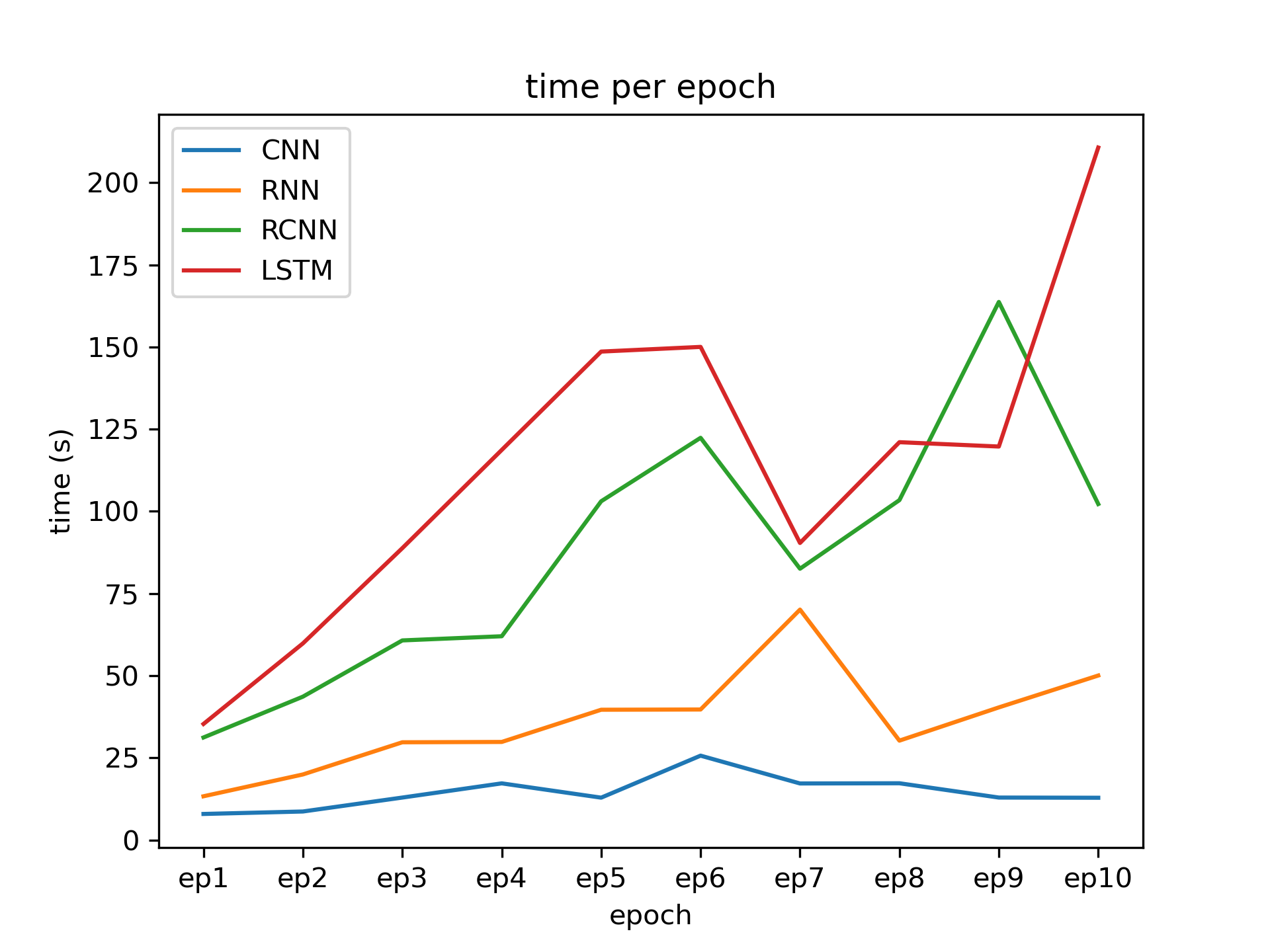
Discussion

By inspection of epoch scores and average scores, the LSTM architecture performs better than the other architectures; when measured for time, however, the CNN has the better performance.

This study is limited by more than a few practical concerns. The two most practical limitations on this study are as follows: the GPU, while a good GPU, is still not an optimized machine for which to perform ML tasks; the flagship 3090 model is a better optimized GPU for such tasks, and the Apple M1 chip is an additional alternative as it is equipped with an NPU (Neural Processing Unit) specifically designed for ML tasks. Additionally, pushing the NLP models to a cluster may also facilitate improved performance. Second: hyperparamter tuning is a difficult (but necessary) part of the machine learning process; these models are optimized to illustrate the project, whereas elsewise greater care with parameter tuning will yield better overall results.

Further improving statistical-based models — Naive Bayes, KNNs, SVMs — can yield great insight into the problem. A very real and valid criticism of ML is that it is an “alchemy” (Flender, 2021; Rahimi & Recht, 2017), in that the scientific rigor of the field betrays the fact “practitioners use methods that work well in practice but are poorly understood on a theoretical level”. This, however, does not defeat the value in exploring models and their respective performances to give insight to their applicability and behavior.

Finally, this project explored accuracy metrics for polarity in sentiment analysis. Nuanced snetiment analyses should probe for — in addition to polarity — feelings and emotions, urgency, and intentionality.

Deep learning is slow, even if we optimize processing units and model architectures. Learning rate is related as the network adapts to new information. Consider the following (original citation of this example is unknown; it is adapted here from a class lecture): suppose a scientist from Mars encounters examples of cats on Earth. Each cat n in the example set N of cats has orange fur. It stands to reason, then, that the Martian scientist will think that cats have orange fur. When trying to identify whether an animal is or is not a cat, our scientist will look for orange fur.

Suppose now that our scientist encounters a black cat, and the representatives of Earth tell the bewildered Martian scientist that that animal is indeed also a cat. This is an example of supervised learning: the Martian scientist is provided with data (a black animal) that is appropriately identified as a cat. Learning rate follows (where “large” and “small” are relative to each other, and their values will depend on the problem being solved):

• Large learning rate indicates that the Martian scientist will realize that “orange fur” is not the most important or useful feature of cats
• Small learning rate indicates that the Martian scientist will simply think that this black cat is an outlier and that cats are still definitively orange

As the learning rate increases, the network will “change its mind”. If it is too high, however, our Martian scientist will think that all cats are black even though more were orange than were black; in other words, our scientist went too far the other way. We want to find a reasonable balance in which the learning rate is small enough that we converge to something useful, but large enough that we do not have to spend unreasonable time training it.

Conclusion

Sentiment analysis does not lack for applicability, and there are many apporaches to the problem in NLP, including statistical ML models and neural network ML models. Investigated here were four neural network models, graded across ten training epochs controlled for validation loss. It was shown that with these architectures, the LSTM model performs best when measured for loss, accuracy, and misclassification rate, while the CNN performs best when measured for training time.

Appendices

Visualization

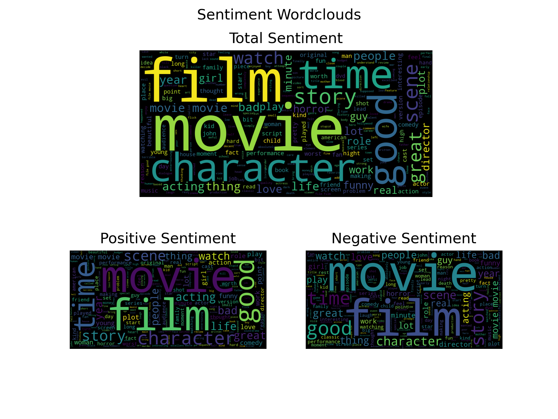
Wordclouds are visualizations of (text) data in which the size of a word represents its frequency or importance in that data. Wordclouds are handy for visualization-at-a-glance, and have the enjoyable consequence of making a report more lively. Inspection of each wordcloud is not immediately useful; overall sentiment cannot be meaningfully extracted by inspection, as no extremes in language can be easily identified.

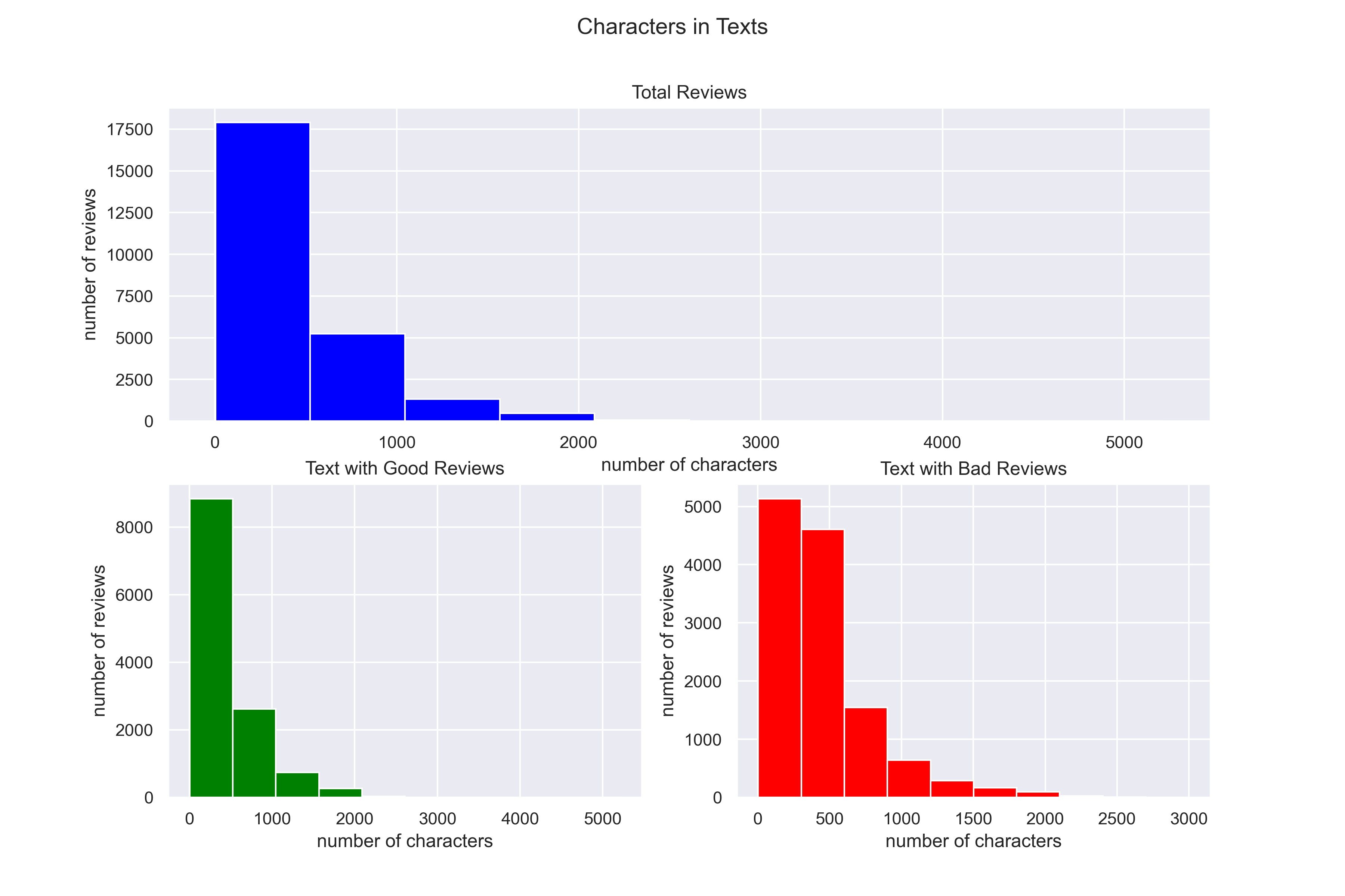
The number of characters in the text refers to simply that: the number of written characters.

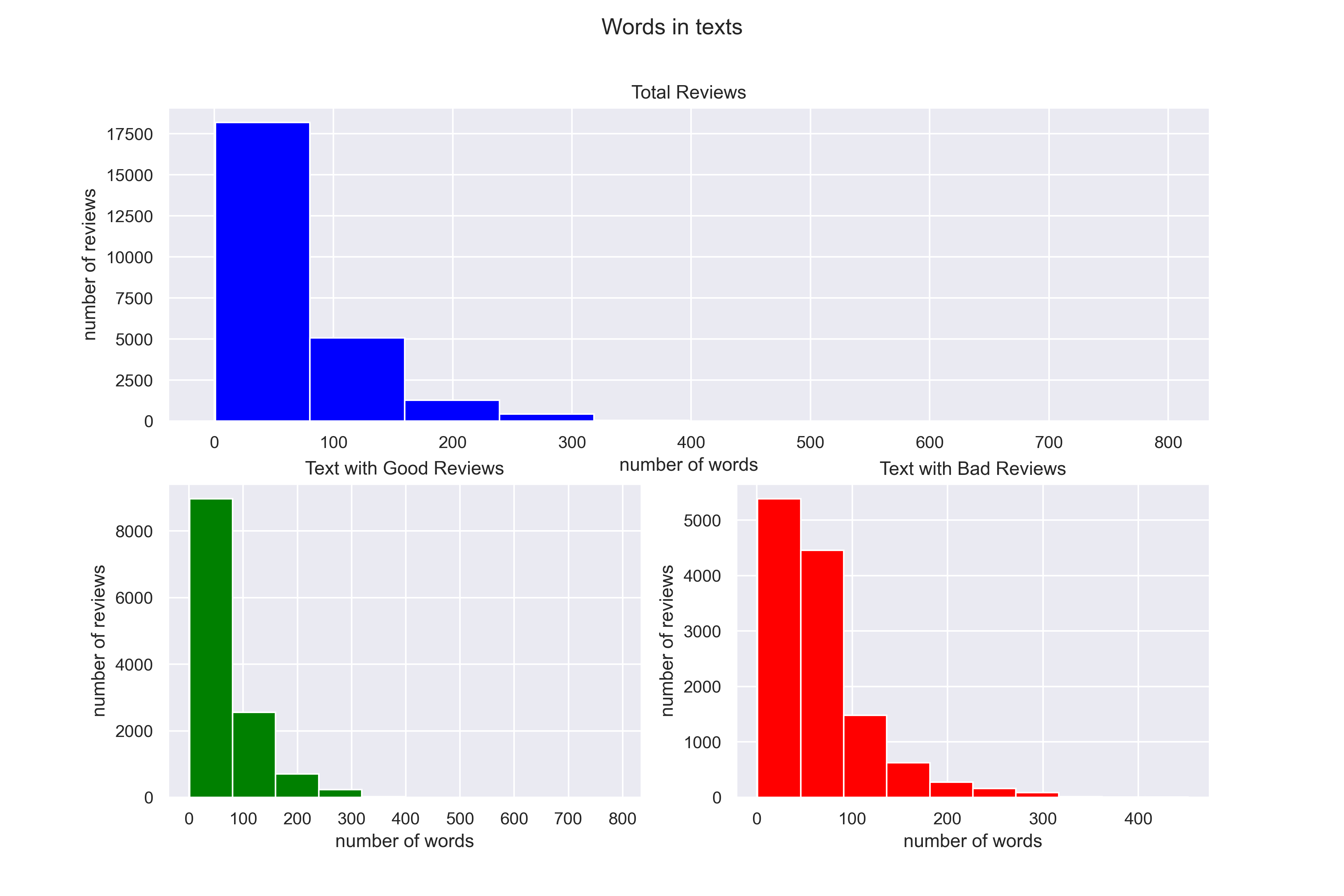
The number of words in the text refers to simply that: the number of words.

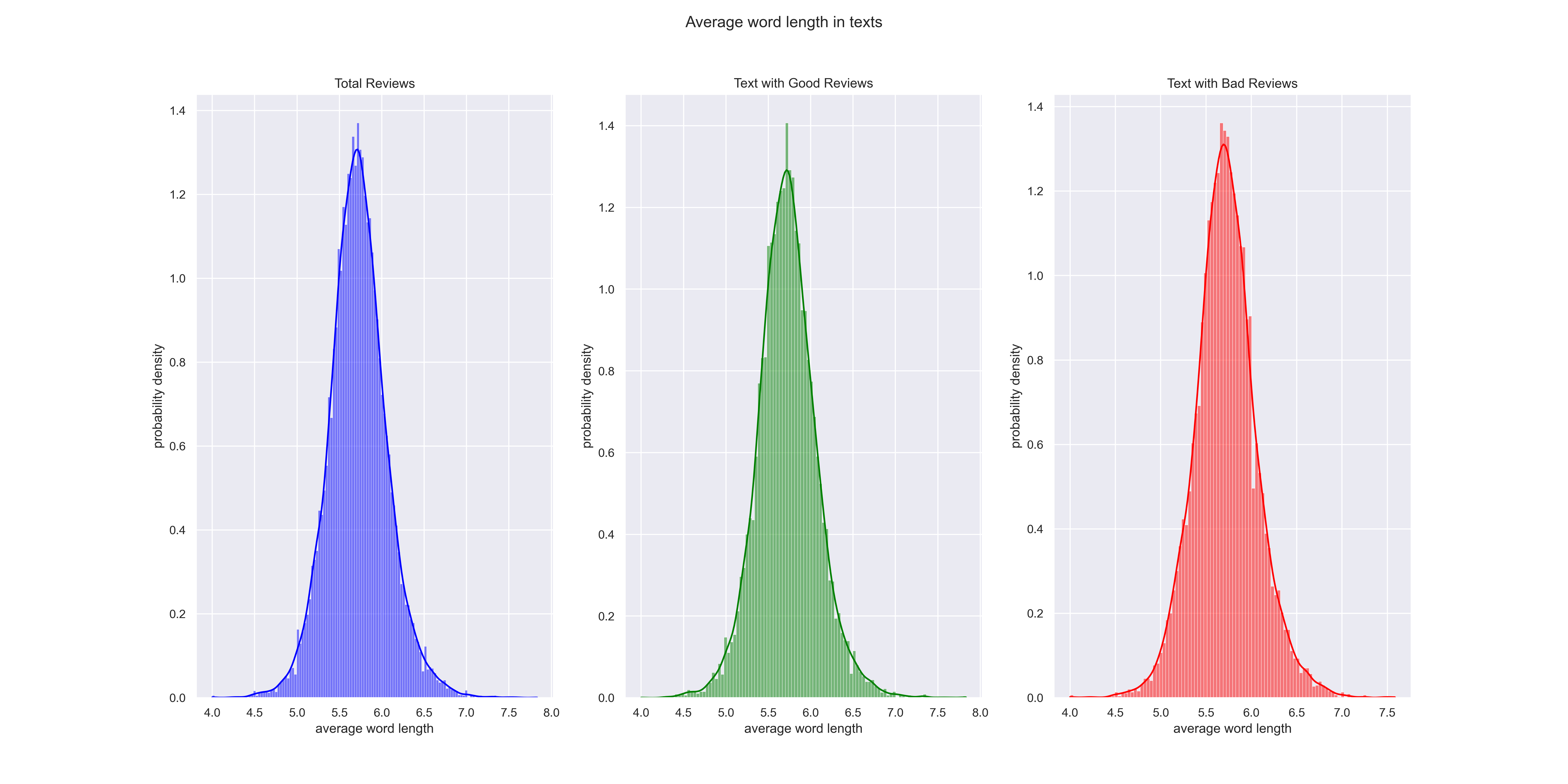
The average word length in the text refers to simply that: the average word length. Note that the average word length is represented by a probability density, the values of which may be greater than 1; the distribution itself, however, will integrate to 1. The values of the y-axis, then, are useful for relative comparisons between categories. Converting to a probability (in which the bar heights sum to 1) in the code is simply a matter of changing the argument stat=’density’ to stat=’probability’, which is essentially equivalent to finding the area under the curve for a specific interval. See this article for more details.

Neural Network Results

Three graphs result from the code that report training time per epoch, metrics (loss, accuracy, and missclassification rate) per epoch without average values, and metrics with average values; for brevity, we report only the CNN metrics graph with averages as a bar graph.

We see that the CNN model performs best at two epochs.

Three graphs result from the code that report training time per epoch, metrics (loss, accuracy, and missclassification rate) per epoch without average values, and metrics with average values; for brevity, we report only the RNN metrics graph with averages as a bar graph.

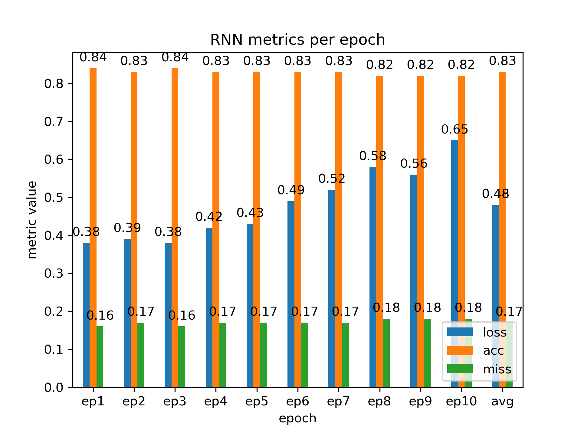
We see that the RNN model performs best at one or two epochs.

Three graphs result from the code that report training time per epoch, metrics (loss, accuracy, and missclassification rate) per epoch without average values, and metrics with average values; for brevity, we report only the RCNN metrics graph with averages as a bar graph.

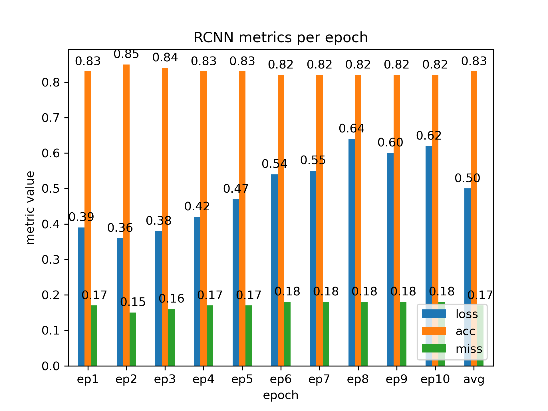
We see that the RCNN model performs best at two epochs.

Three graphs result from the code that report training time per epoch, metrics (loss, accuracy, and missclassification rate) per epoch without average values, and metrics with average values; for brevity, we report only the LSTM metrics graph with averages as a bar graph.

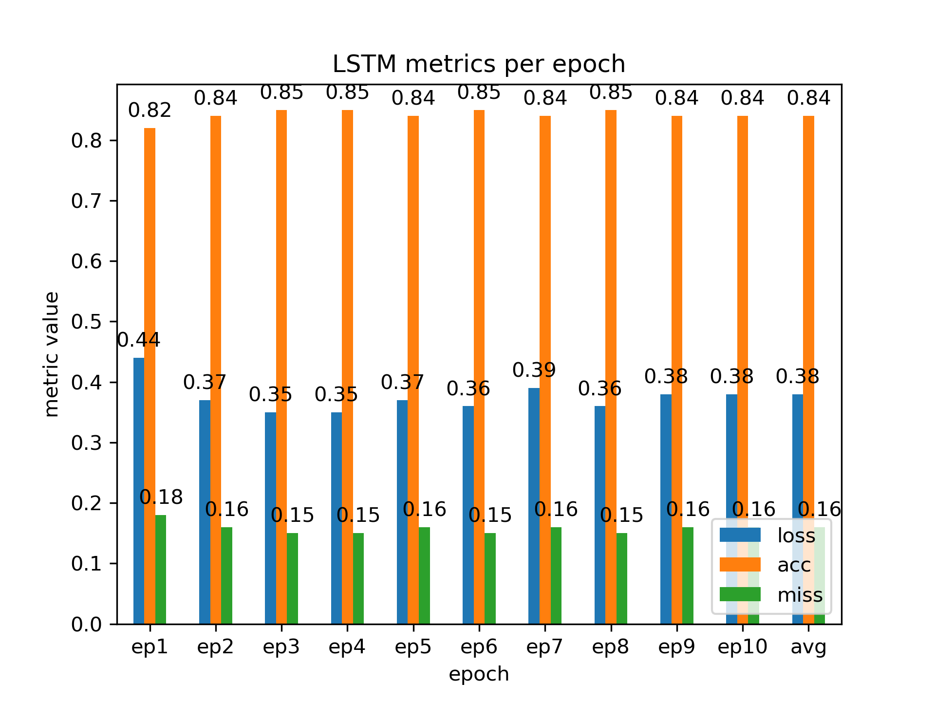
We see that the LSTM model performs best at three or four epochs.

Bibliography

Bodapati, J., Veeranjaneyulu, N., & Shaik, S. (2019). Sentiment analysis from movie reviews using lstms. Ingénierie des systèmes d information, 24, 125–129. https://doi.org/10.18280/isi.240119

Flender, S. (2021). Machine learning: Science or alchemy? https://towardsdatascience.com/machine-learning-science-or-alchemy-655bea25b227

Hoang, M., Bihorac, O. A., & Rouces, J. (2019). Aspect-based sentiment analysis using BERT. Proceedings of the 22nd Nordic Conference on Computational Linguistics, 187–196. https://aclanthology.org/W19-6120

Jang, B., Kim, M., Harerimana, G., Kang, S.-u., & Kim, J. W. (2020). Bi-lstm model to increase accuracy in text classification: Combining word2vec cnn and attention mechanism. Applied Sciences, 10(17). https://doi.org/10.3390/app10175841

Kelleher, J. D., Namee, B. M., & D’Arcy, A. (2015). Fundamentals of machine learning for predictive data analytics (1st). The MIT Press.

Maas, A. L., Daly, R. E., Pham, P. T., Huang, D., Ng, A. Y., & Potts, C. (2011). Learning word vectors for sentiment analysis. Proceedings of the 49th Annual Meeting of the Association for Computational Linguistics: Human Language Technologies, 142–150. http://www.aclweb.org/anthology/P11-1015

Rahimi, A., & Recht, B. (2017). Reflections on random kitchen sinks. http://www.argmin.net/2017/12/05/kitchen-sinks/